Persistency Checking of Gaussians
Steve Fulton
Thus far, approximately 20 million distinct Gaussians
have passed data integrity testing.
For these signals we standardized the score
such that there were on average an equal number of Gaussians in each workunit group
with scores greater than or equal to 1.0. (See "An Explanation of Score Correction" below for details.)
This standardization left 1.25 million Gaussians of interest to be examined further.
From these signals we then determine which Gaussians have been detected in the same location of the sky on multiple occasions.
This process is called persistency checking.
For our first pass through the data, we performed an analysis with very
restrictive bounds on matches. Gaussians were considered matches if they conformed to the following criteria:
The right ascension and declination restrictions approximate
the beam size at Arecibo. Barycentric frequency is used to correct for the
Doppler effects caused by Earth's rotation and its orbit around the sun.
The barycentric frequency divergence across a
beam at Arecibo is approximately 125Hz. The final bounds on the time remove the
possibility of detecting multiple images of the Gaussian from a single observation.
1,397 multiplets (multiply-detected Gaussians) meet the above criteria.
Future analyses will identify the best candidates from this group.
An Explanation of Score Correction
 The SETI@home feed at Arecibo moves at varying rates as the opposing feed tracks objects in the sky. At faster rates, the SETI@home
client obtains fewer points over a fixed angular separation. With fewer data points false detections are more likely, and hence
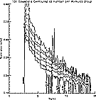
the client detects more Gaussians and higher scoring Gaussians as the rate of telescopic movement increases. (See Figure 1 on the right, where (uncorrected) Gaussian score is on the y-axis and the width of the Gaussian (sigma) is on the x-axis - click on it to enlarge.)
This slew-rate detection dependence creates problems when looking for persistent signals. Persistency
detection assumes that there is an equal chance of detecting a Gaussian each time
the telescope passes a given point in the sky; the analysis uses this assumption to rank persistent multiplets
and reject temporal rfi. To fix the problem, we corrected the factors
used to calculate score such that the number of signals in a workunit group
with significant scores is constant across slew rate.
 Statistically, the score of a Gaussian is defined as the peak-power/chi-square.
The chi-square is a measure of the Gaussian's fit (i.e., how well the signal matches a classic Gaussian curve, with a lower score representing a better fit).
Since both the peak-power and chi-square terms reported back by the
client were dependent on the telescope slew rate,
a simple correction function was needed for each of the terms.
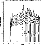
The resulting "flattened" peak power and chi-square were used to define the new
(corrected) score (Figure 2 on the left - click on it to enlarge). (Note that the Y-axis in Figure 2 is mislabelled--instead of "Score uncorrected", it should read "Score corrected".)
The normalization was set so that on average each workunit group would
have 4 Gaussians with a score 1.0 or greater. This score approximates a
chi_square cutoff of 8.8 (uncorrected) at low slew rates, which is the
threshold used by the client.
Return to Science Newsletter main menu
| 

