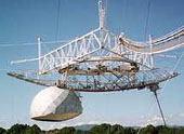
In Newsletter 18 we discussed how SETI@home observes known sources of noise (such as the Crab Nebula) to establish that we are accurately recording where our receiver is pointing. You may wonder why we're so concerned about maintaining positional accuracy—the problem relates to the fact that the SETI@home receiver at Arecibo is calibrated independently from the receivers of other projects.

The receivers for most projects are located in the geodesic dome of the platform suspended 500 feet above the telescope dish. (The platform and dome are pictured at right.) The dome is mobile and can be adjusted to maintain precise accuracy as the telescope tracks celestial objects. SETI@home's receiver, however, is located on the opposite end of the platform, in "Carriage House 1" (located at the base of the long, downward-pointing antenna to the right). Carriage House 1 is also adjustable, but independent of the geodesic dome. We therefore take great care to monitor our pointing accuracy; we may have error offsets at Carriage House 1 even if the geodesic dome is perfectly calibrated.

The geodesic dome and Carriage House 1

Azimuth and altitude

From our observation point at Arecibo, the celestial sky appears as a giant circle overhead, bounded by the horizon. When the telescope observes a position in space, SETI@home's accuracy might have an error in one or two dimensions; the receiver might be collecting data slightly above/below or to the left/right of where we think we're observing.

Normally we document celestial positions using right ascension (RA) and declination (Dec) parameters. This coordinate system (called the Equatorial coordinate system) is anchored to the sky such that stars and other celestial locations always have the same coordinates regardless of time or location of observation. (For example, the Crab Nebula has an RA of 5 hours and a Dec of 22 degrees at all times of the day, and from all observation points on Earth.)

However, when we test the accuracy of our positioning, we want to make adjustments based on where the telescope is physically pointing relative to its horizon, and the Equatorial coordinate system doesn't provide this information. Therefore, using RA, Dec, time, and the latitude and longitude of the telescope itself, we convert our position data to the Horizontal coordinate system. Using this coordinate system, celestial objects will change coordinates as they move across the sky, but the positioning of the telescope remains consistent. The Horizontal coordinate system describes the celestial sphere in terms of azimuth and altitude. As shown in the figure below, azimuth is the angle of an object around the horizon, while altitude (or "elevation") is the angle of an object above or below the horizon.

Choosing sources for position testing

Once our data is described in terms of azimuth and altitude, we can begin tracking known sources of noise (like the Crab Nebula) as they sweep across Arecibo's telescope beam. Sometimes a noise source will go right through the beam; at other times there might be a near miss. If we obtain enough of these "sweeps", we can average across them to discover any location differences between our reported data and the true location of the source. However, since the telescope passes a particular source only a handful of times at best in our data, we need to investigate a large number of sources together to calculate reliable location offsets.

79 sources in total were used to compare SETI@home HI absorption data to the data established by a previous HI absorption study. Below are hydrogen absorption graphs from two of these sources (named 3C133 and 3C409). The white line in each graph plots the level of hydrogen absorption as the source (and all signals within .2 degrees of that source) passes across Arecibo's telescope beam. In the example of 3C133, hydrogen absorption maxes out at around spectrum number 25, meaning that at this point the source approaches our telescope beam most closely. These plots are made using data from several different days, so we see several passes over 3C409.

Beam Pattern

To take an "overhead view" of the preceding two graphs, we can plot the location of each data point on altitude and azimuth axes and make the most hydrogen-absorbed data appear warmer in color (with white as the hottest, most absorbed data, meaning that the white points are closest to strong noise sources). Below is such an overhead graph, representing data from both of the above graphs along with data from two additional sources. Plotting the data from these 4 sources on a alt/az square seems to show a consistent beam pattern, as we see below.

Beam Fit Results

Given the varying absorption patterns of each of the four "sweeps", we can determine the center of absorption (or the location of the source causing the most hydrogen absorption) by making an iterative least-squares best-fit calculation. The graph below displays a dotted circle around this center of absorption, showing where our beam is actually recording. A perfectly calibrated beam would have its center of absorption in the exact center of the graph, at the point of origin. Clearly, our graph shows a calibration offset in terms of azimuth (centered high on the y-axis). The exact offsets were calculated to be the following:

With this information we correct our coordinate data to accurately locate the signals SETI@home detects.

Return to Science Newsletter main menu